More simulations

In the previous tutorial we only simulated simple 1D diffusion processes. Here, we show more examples of simulations with different dynamics, illustrating in particular the generic class stochrare.dynamics.diffusion.DiffusionProcess.

2D Diffusions: gradient dynamics

Let us start with basic diffusion processes in 2D: the Wiener process and the Ornstein-Uhlenbeck process.

import numpy as np
import matplotlib.pyplot as plt
from stochrare.dynamics.diffusion import Wiener, OrnsteinUhlenbeck

np.random.seed(seed=100)

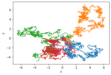
ax = plt.axes(xlabel=r'$x$', ylabel=r'$y$')
for _ in range(4):
    t, x = Wiener(2).trajectory(np.array([0., 0.]), 0., dt=0.01)
    ax.plot(x[:, 0], x[:, 1])

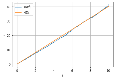
time, dist2 = zip(*[(t,r) for t,r in Wiener(2).sample_mean(np.array([0.,0.]), 0., 1000, 1000, dt=0.01,
                                                           observable=lambda x, t: x[0]**2+x[1]**2)])
ax = plt.axes(xlabel=r'$t$', ylabel=r'$r$')
ax.grid()
ax.plot(time, dist2, label=r'$\langle \Delta x^2 \rangle$')
ax.plot(time, 4*np.array(time), label=r'$4Dt$')
ax.legend();

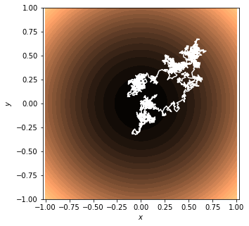
model = OrnsteinUhlenbeck(0,1, 0.1, 2)
xvec = np.linspace(-1., 1.)
yvec = np.linspace(-1., 1.)
potential = np.array([model.potential(np.array([x, y])) for x in xvec for y in yvec]).reshape(50, 50)
fig = plt.figure(figsize=(5, 5))
ax = plt.axes(xlabel=r'$x$', ylabel=r'$y$')
ax.axis('equal')
ax.contourf(xvec, yvec, potential, 30, cmap='copper')
t, x = model.trajectory(np.array([0., 0.]), 0., T=2, dt=0.001)
ax.plot(x[:, 0], x[:, 1], color='white');

Langevin equation

Now we simulate the Langevin dynamics:

\[\dot{x}=p/m, \quad \dot{p}=-V'(x)-\gamma p +\eta(t),\]

with a harmonic potential \(V(x)=x^2/2\) and \(\mathbb{E}[\eta(t)\eta(t')]=D\delta(t-t')\).

from stochrare.dynamics.diffusion import DiffusionProcess
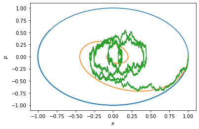
gamma = 0
def langevin(gamma, D):
    return DiffusionProcess(lambda X, t: np.array([X[1], -X[0]-gamma*X[1]]),
                            lambda X, t: np.array([[0., 0.], [0., D]]))

Without friction and noise (\(\gamma=D=0\)), the system is Hamiltonian and \(H=x^2+p^2\) is conserved. Adding some friction \(\gamma >0\), the system relaxes towards equilibrium in a spiraling motion, because of inertia. With noise, we inject energy randomly in the system, and the stationary distribution spreads over a region of phase space centered on the origin.

xvec = np.linspace(-1., 1.)
pvec = np.linspace(-1., 1.)
ax = plt.axes(xlabel=r'$x$', ylabel=r'$p$')
t, x = langevin(0, 0).trajectory(np.array([1., 0.]), 0., T=10, dt=0.001)
ax.plot(x[:,0], x[:,1]);
t, x = langevin(0.5, 0).trajectory(np.array([1., 0.]), 0., T=10, dt=0.001)
ax.plot(x[:,0], x[:,1]);
t, x = langevin(0.5, 0.2).trajectory(np.array([1., 0.]), 0., T=20, dt=0.001)
ax.plot(x[:,0], x[:,1]);